What is an efficient way to sample an agricultural field?
Sampling on an agricultural field is often done in a grid. I do not like this concept because the shortest distance between two sampling points is the actual grid size. For example if a soil sample is taken in a 50m grid the shortest distance is therefore also 50m in between the points. When I then plot a variogram and fit a function to it the smallest lag will also be 50m. Consequently, I do not know how a soil parameter changes on smaller distances than the 50m.
Contrary to a grid sampling strategy one could also randomly sample across a field. But then there is the risk that areas are over- or under-sampled. I therefore like the idea of stratified sampling. The field is partitioned into strata and in each stratum the one or more sampling locations are chosen randomly.
The solution: stratified sampling in R
This can be done nicely in R. All that is necessary is a polygon shape file in WGS84 projection that outlines the sampling site. First I load the required libraries for managing a shape file (rgdal), perform the stratified sampling (spcosa), and for solving the traveling salesman’s problem (TSP).
require(TSP)
require(spcosa)
require(rgdal)
The next step is to load the shape file into R. This is done with the readORG command. The command has to parameters, the first is the absolute path to the file, and the second is the shape file itself. In my case the name of the shape file is “boundaries.1d”.
reagan<-readOGR(dsn="/Users/knappi/projects/DeeFarm/GIS/R",layer="boundaries.1d")
Then I perform the actual stratification and sampling
# set seed to be able to replicate results
set.seed(314)
myStratification <- stratify(reagan, nStrata = 50, nTry = 3,equalArea = T)
# sample two sampling units per stratum
mySamplingPattern <- spsample(myStratification, n = 2)
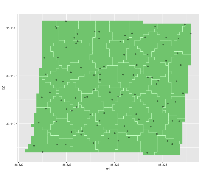
I set the number of strata to 50 and I also set equalArea to TRUE. Important: this only worked for me after I removed the projection file from the shape file folder. I then sample twice per stratum. Now let’s see how this looks like.
plot(myStratification, mySamplingPattern)
This looks nice! The next step is to extract the coordinates and then save them as a csv file:
data<-mySamplingPattern@sample
# access the coordinates of the sampling points and save to csv.
samples<-as.data.frame(data@coords)
names(samples)<-c("longitude","latitude")
write.csv(samples,file="SamplingPoints.csv",row.names = F)
Now to sample the 100 locations on this field still seems to be very inefficient. I therefore use the TSP package to apply an algorithm that solves the traveling salesman problem:
# create distance matrix
d.s<-dist(samples)
# create TSP object
tsp.s<-TSP(d.s)
tsp.s<-insert_dummy(tsp.s, label = "cut")
tour.s<-solve_TSP(tsp.s)
path <- cut_tour(tour.s, "cut")
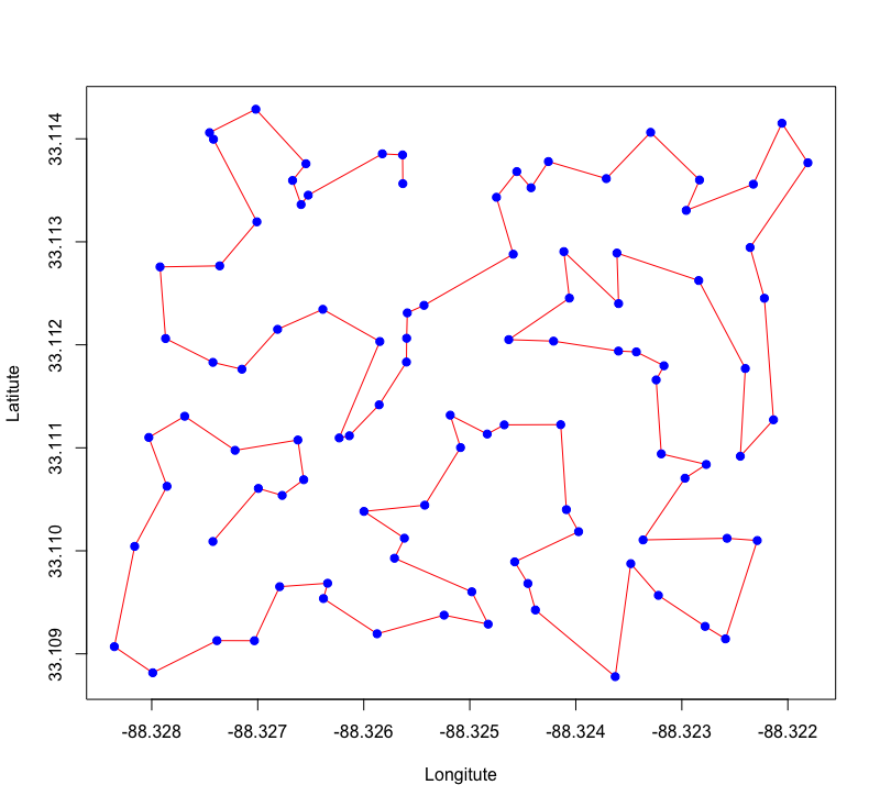
I have stitched together these lines based on this article. Let’s see how the suggested path looks like.:
plot(data@coords[path,],type="l",col="red",pch=19,
     xlab="Longitute",
     ylab="Latitute")
points(data@coords[path,],col="blue",pch=19)
The suggested solution seems to be an efficient way to sample the field. The final step is to save an updated list of the sampling locations in the order of the red line:
samples<-samples[path,]
write.csv(samples,file="SamplingWayPoints.csv",row.names = F)
This csv file can now be added to a GPS device as a waypoint file and the field can be samples accordingly.


